AirSketcher Manual

Welcome to the AirSketcher user manual. This guide will walk you through every essential and advanced feature of the software for setting up and running CFD simulations with ease.

Introduction

AirSketcher is a lightweight 2D CFD simulation and visualization tool built for rapid design exploration and intuitive analysis. Unlike traditional CFD platforms that require extensive setup, meshing, and scripting, Air Sketcher simplifies the process — just draw your domain, press run, and see results.

Designed for speed and usability, it enables engineers, designers, educators, and students to test airflow concepts on the fly — whether across mechanical structures, ventilation layouts, or environmental enclosures.

With built-in modules, Air Sketcher delivers:

• A fast steady-state CFD solver with adaptive meshing

• Real-time streamline and particle tracking visualizations

• Performance reporting based on selected regions of interest

• One-click PDF report generation with detailed summaries

• Direct input via mouse or stylus for sketch-based geometry creation

No CAD. No complex setup. No barriers. Just insight — fast.

Installation

To install AirSketcher, follow these simple steps:

1. Download the installer

Locate and run the provided setup.exe file.

2. Activate with your license key

During the first launch, you’ll be prompted to enter the license key you received after purchase.

3. One-time online verification

The software will briefly connect to the server to verify your license. If the key is valid, a local license file will be generated and saved on your machine.

4. Offline usage enabled

After activation, AirSketcher will no longer require an internet connection. You can run it offline anytime.

💡 *Make sure to keep your license key in a safe place for future reference

System Requirements

To ensure smooth operation, AirSketcher requires the following minimum system specifications:

🖥️ Operating System

• Windows 10 or later (64-bit)
• macOS & Linux: Support planned for future releases

⚙️ Hardware

• CPU: Dual-core processor or better
• RAM: 4 GB minimum (8 GB or more recommended)
• Storage: ~3 GB for installation
• Graphics: Integrated GPU is sufficient (no high-end GPU required)

🌐 Internet

• Required only during the first activation to verify the license key.
• An internet connection is used to detect version updates.
• No internet connection is needed for core features after successful activation.

✅ AirSketcher is optimized for lightweight 2D simulations and user-friendly visualization. It does not require a high-end workstation. ## Quick Start Guide

Follow these steps to run your first CFD simulation in AirSketcher:

Launch the Application

Double-click the AirSketcher icon. The main interface will open with a clean canvas and controls on the left.

Set the Wind Speed

• At the top-left, adjust the Wind Speed (in m/s).
• Default is 5 m/s — suitable for general testing.

Define Your Simulation

Domain

• Use the drawing tools to sketch obstacles (e.g. walls, buildings, airfoils).

• Or import geometry from the Image Processor on the right panel.

Expert Options

Click Expert Options ▶ to access advanced controls like:

• Gravity Enabled

• Wind Tunnel Mode

• Ground Friction

• ABL Inlet

• AMR Enabled

• Scale Input Wind Speed

• Set Domain Height

• Porous Zones / Blowers

Run the Simulation

• Click Run.
• The solver will compute flow behavior in real-time.
• You’ll see the running residual plots, system metrics, and optional velocity vector overlays.

Understanding the Solver Phases

AirSketcher uses a hybrid approach, automatically transitioning between two distinct simulation phases. Understanding these phases will help you know exactly when to record your data and when to stop the simulation.

Phase 1: Pseudo-Transient (Mean Flow & Force Stabilization) When you first click Run, the solver focuses on quickly establishing the basic, stable flow field around your obstacles. During this phase, it applies numerical techniques to force the mass flow to balance and the overall pressure field to settle.

Phase 2: Full Transient (Wake Phase & Vortex Shedding)

Once the mean flow achieves stability, the solver automatically disables its artificial stabilization controls—specifically the mass flow “outlet servo” and momentum correction. It turns these off because artificial constraints suppress natural fluid motion. Instead, it activates the “Wake Phase” and introduces slight physical perturbations into the flow. This allows natural, time-dependent fluid phenomena—like the von Kármán vortex street—to develop behind your objects.

Monitoring Convergence & UI Indicators

Watch the Residuals panel in the plot window. It shows how stable and balanced the numerical solution is while the simulation is running. The colored LED dots give a quick health check of the flow calculation.

What are residuals?
A residual is a measure of how much the solution is still changing from one solver iteration to the next.

In simple terms:
large residual = the flow field is still changing
small residual = the flow field is becoming stable

AirSketcher tracks residuals for the main solved fields: horizontal velocity, vertical velocity, and pressure.

Residuals do not directly mean “percent error compared with reality.” Instead, they show whether the CFD equations are settling into a consistent solution. A simulation can start with high residuals because the solver is still building the flow field from the initial condition. As the flow stabilizes, residuals should generally decrease.

Residuals: Vx, Vy, and Pressure

The residual indicators monitor three key fields:

• Vx residual: Change in horizontal velocity from one iteration to the next.
• Vy residual: Change in vertical velocity from one iteration to the next.
• Pressure residual: Change in the pressure correction field from one iteration to the next.

Use the LED colors as a quick guide:

• Residuals: Vx, Vy, Pressure
  • 🟢 Green (< 0.003): Excellent convergence. The flow equations are well-balanced and the solution is stable.
  • 🟠 Orange (< 0.009): Acceptable or transitioning. The solution is improving, but the flow is still adjusting.
  • 🔴 Red: High residuals. This is normal at the beginning of a run, after large geometry changes, or during sudden wake transitions.

Practical interpretation
If the residuals are dropping and staying low, the solution is converging.
If the residuals stay high, grow continuously, or spike repeatedly, the simulation may be unstable or the flow may still be developing.

Mass Flow Balance

Mass Flow Balance checks whether the amount of air entering the domain is close to the amount leaving it.

Look for:

• Mass Flow Balance ≥ 95.0%

This means the inlet and outlet flow rates are reasonably balanced.

Why this matters
For a stable CFD solution, air should not artificially appear or disappear inside the domain. A high mass-flow balance indicates that the solver is conserving flow well.

Typical interpretation:

• ≥ 95%: Good balance for most visual and design studies.
• Near 100%: Excellent balance.
• Low balance: The simulation may still be developing, or the setup may need adjustment.

If mass balance remains poor, try:

• reducing inlet speed;
• enabling Refine Flow;
• checking for overly tight geometry gaps;
• increasing domain height;
• simplifying very sharp or noisy obstacle boundaries.

ΔCd: Change in Drag Coefficient

ΔCd shows how much the drag coefficient is still changing as the simulation runs.

This is especially important when you are using AirSketcher to estimate aerodynamic forces such as drag and lift.

• ΔCd: Change in Drag Coefficient
  • 🟢 Green (< 0.05%): Aerodynamic forces have stabilized. This is the best time to record Cd and Cl values.
  • 🟠 Orange (< 1.0%): Forces are approaching a stable value but may still be changing.
  • 🔴 Red: Forces are still fluctuating. Wait longer before recording final aerodynamic values.

Practical interpretation
Low residuals tell you the flow equations are stable.
Good mass balance tells you air is conserved.
Low ΔCd tells you the aerodynamic force result has stopped changing significantly.

Recommended Workflow

1. Start the simulation and allow the residuals to drop from their initial high values.
2. Watch for Vx, Vy, and Pressure residuals to turn green or remain consistently low.
3. Confirm that Mass Flow Balance reaches at least 95.0%.
4. If you need aerodynamic coefficients, wait until ΔCd turns green.
5. Record final values only after the residuals, mass balance, and ΔCd are all stable.

Important note
A short red or orange period is normal at startup. The key is the trend. A healthy simulation should move toward lower residuals, better mass balance, and smaller force changes over time. Watch the Residuals panel on your plot window. The colored “LED” dots provide a quick health check of your simulation:

• Residuals (Vx, Vy, Pressure):
  • 🟢 Green (< 0.003): Excellent convergence. The flow equations are well-balanced.
  • 🟠 Orange (< 0.009): Acceptable/Transitioning.
  • 🔴 Red: High residuals. (Normal at the very beginning or during sudden wake transitions).
• Mass Flow Balance: Look for this to reach ≥ 95.0%. This means the amount of air entering the domain matches the amount leaving.
• ΔCd (Change in Drag Coefficient):
  • 🟢 Green (< 0.05%): The aerodynamic forces on your object have completely stabilized.
  • 🟠 Orange (< 1.0%): Forces are getting close to a final value.
  • 🔴 Red: Forces are still fluctuating.

When to Record Aerodynamic Data (Cd & Cl)

If your primary goal is to find the Drag (Cd) and Lift (Cl) coefficients of your design, you should pay attention to Phase 1.

1. Wait for the “Converged” Message: When residuals drop and mass balance is achieved, AirSketcher will notify you that the flow field has converged.
2. Wait for the “ΔCd Stabilised” Pop-up: As the simulation continues, the solver continuously monitors the change in your drag coefficient. Once |ΔCd| stays below 0.05% for several consecutive checks, a message will pop up saying: “ΔCd has gradually reached ~0%. Aerodynamic forces appear stable.”
3. Record Your Data: This is the optimal time to record your Cd and Cl values. Once the simulation enters the Wake Phase (Phase 2), these values will naturally begin to oscillate as vortices shed off the back of your object.

When to Stop the Simulation

• To get aerodynamic data: You can safely click Stop right after you record your Cd and Cl values from the “ΔCd Stabilised” prompt.
• To observe wake behavior: If you want to see how the air tumbles and sheds behind your object, leave the simulation running. Once you see the “🌪️ WAKE ENABLED” toast notification, the solver is actively cultivating the wake. Allow it to run for a while longer to watch the beautiful, dynamic vortex shedding develop in the visualizer. Stop it whenever you are satisfied with the visual results.

View Results

Once the simulation is complete, explore the results using the top results panel:

• Streamlines – Visualize flow patterns and direction.

• Static Pressure – View pressure distribution in the domain.

• Particle Tracking – Simulate how particles would move through the flow.

• Line Probe and x–y Plots – Analyze flow variables (e.g., velocity, pressure) along a defined line in the domain.

• Report – Auto-generate a summary report including settings and key flow data.

• Qi-Flow – Blends CFD with Feng Shui to assess air harmony, clarity, and comfort.

Each result opens in a new window with zoom, colorbars, tooltips, and export options.

Save Case and Data

Export your processed simulation as a .pkl file using the Save button if needed for post-processing or external tools.

✅ You’re now ready to explore more advanced configurations!

User Interface Overview

When you launch AirSketcher, you’ll see the interface divided into key functional areas:

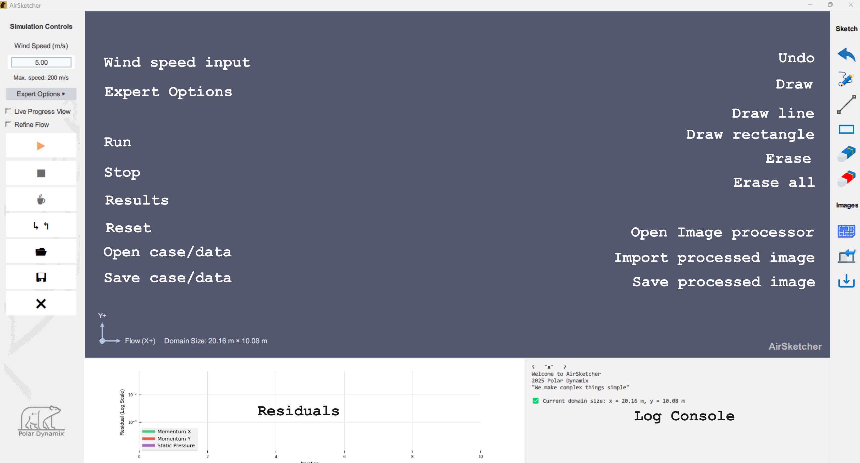
Left Panel — Simulation Controls

This is where you control how the simulation runs:

• Wind Speed (m/s): Set the incoming flow velocity.
  

• Expert Options ▶: Opens advanced settings (e.g., ABL, gravity, AMR).

• Live Progress View shows a real-time visual summary of the simulation, updated every 200 iterations. It helps users monitor airflow behavior and simulation quality as it evolves.

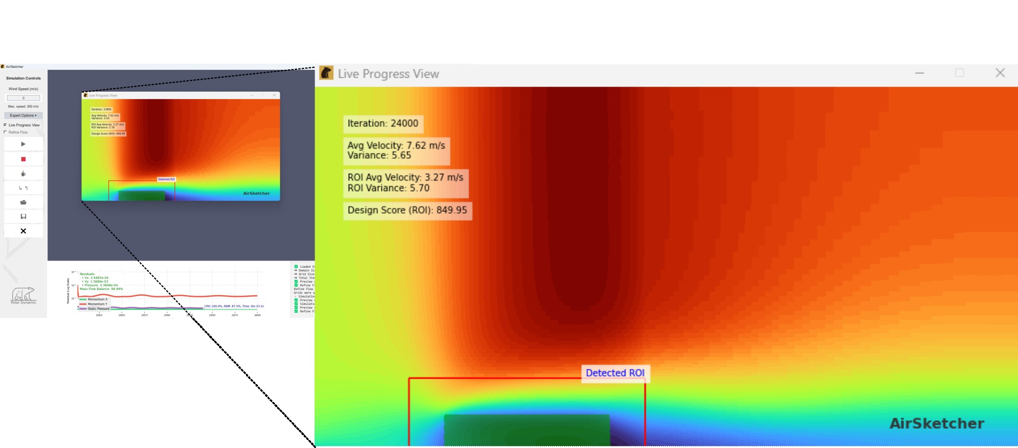
The preview includes:

• Number of iterations
• A velocity contour map over the domain (masked by obstacles)
• Visual overlays for any porous or blower zones (if defined)
• A red outline for the Region of Interest (ROI), if detected
• Live flow statistics:
  • Average velocity and variance over the full domain
  • ROI-specific velocity stats when ROI is active

It also calculates a Design Score using the following formula:

$$ \text{Design Score} = \frac{100 \cdot \overline{V}_{\text{ROI}}}{1 + 0.5 \cdot \sigma^2_{\text{ROI}}} $$ where:

• $\overline{V}_{\text{ROI}}$ is the average velocity inside the ROI
  
• σ_ROI² is the velocity variance inside the ROI

The Design Score rewards airflow that is both strong and consistent within the target region. Higher scores indicate faster average velocity with lower variation — ideal for achieving stable, efficient ventilation performance.

• Refine Flow automatically adjusts the simulation to maintain numerical stability when the vertical grid size (Ly) is too fine for the given inlet velocity.

This is based on the Courant–Friedrichs–Lewy (CFL) condition, which limits the time step for stability:

$$ \Delta t \leq \frac{Ly}{u} $$ Where:

• Δt — simulation time step
  
• Ly — vertical grid spacing
  
• u — inlet velocity

If the flow is slow and the grid is very fine, the required time step Δt becomes extremely small. If the simulation does not reduce the time step accordingly, it may become unstable or diverge.

To prevent this, Refine Flow automatically activates when Ly is smaller than a safe threshold for the current velocity.

Users may still turn Refine Flow ON or OFF manually. However, if it is turned ON automatically, the system will not disable it without user input.

• Run / Stop / Results:
  • Run: Start or continue simulation.
  • Stop / Pause: Temporarily halt computation.
  • Results: Access analysis tools after a run completes.
• Case and Data:
  • Reset Data: Clears current simulation data to start fresh.
  • Load / Save: Load or save a working simulation file.
  • Exit: Close the application.

Right Panel — Sketch and Image Tools

Sketch & Tools

From top to bottom:

• Undo: Reverse or reapply your latest actions.
  
• Draw: Create geometry using freehand or brushes.
  
• Draw Line: Click to draw straight lines.
  
• Draw Rectangle: Draw rectangle shapes.
  
• Eraser: Remove selected geometry.
  
• Eraser All: Remove all geometry on the canvas.

Image Tools

Bottom Three Icons:

• Image Processor: Launch the Image Processor and Windrose Locator module.
  
• Import Processed Image: Load the processed image from the Image Processor back onto the canvas.
  
• Save Processed Image: Save the currently drawn domain/obstacles as a temporary file named saved_drawing.pkl (used for restarting or post-processing).

Center Canvas — Drawing & Simulation View

This is your main workspace:

• Displays the geometry, flow domain, velocity arrows, and simulation progress.
  
• Shows directional axes: X (Flow) →, Y ↑
  
• When results are available, this area displays streamlines or pressure contours.

Bottom — Residuals and Log Console

• Residual Plot (Log Scale): Tracks solver convergence over time for:
  • Momentum X
  • Momentum Y
  • Static Pressure
• Log Console (Right Corner): Status updates, grid info, AMR messages, etc.

Simulation Setup

Setting up your simulation involves defining the environment where air will flow. This includes specifying the domain size, placing obstacles, and applying boundary conditions. AirSketcher offers an intuitive interface to guide you through each step.

Setting Domain Size

To define the vertical size of your simulation area:

1. Click on “Set Domain Height (Y)” in the Expert Options panel.
   
2. Enter your desired height value in meters.
   
3. The domain length (X) is automatically scaled based on the canvas width.

💡 Tip: Ensure all obstacles are placed within the domain and away from boundaries to minimize their impact on flow and avoid simulation errors.

Defining Obstacles

Obstacles represent solid objects like buildings, walls, or terrain features that influence airflow.

• Drawing Tools: Use the right-hand toolbar to draw directly on the canvas.
  
• Eraser Tool: Remove unwanted geometry or correct mistakes.
  
• Import Geometry: Load shapes or drawings created earlier. See Image Processor for more information.

📝 Note: Ensure obstacles form closed loops to be treated as solids.

Expert Options

These expert settings give you deeper control over simulation physics and performance. To reveal them, click the Expert Options ▶ button under the Wind Speed setting.

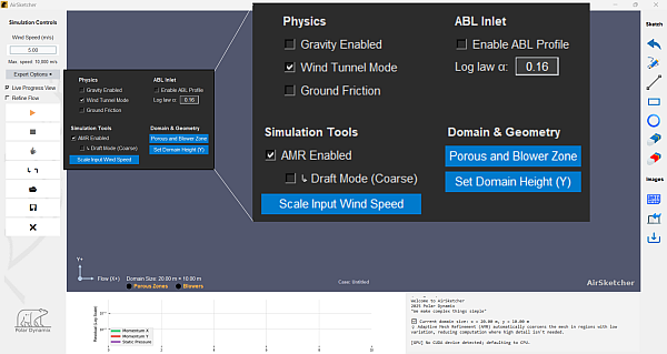
Gravity Enabled

Applies downward gravity to the airflow. Useful for buoyancy-driven flows (e.g., warm air rising) or terrain-influenced drafts. When disabled, the simulation assumes horizontal-only flow without vertical buoyancy effects.

🌬️ Wind Tunnel Mode

This mode applies slip-wall (symmetry) boundary conditions to the top and bottom walls of the simulation domain, simulating a confined but frictionless tunnel.

Slip Wall / Symmetry Boundary means:

• No flow through the wall: Perpendicular velocity is zero (v = 0).
• Frictionless sliding: No shear stress along the wall (zero gradient of parallel velocity and pressure).

Use this for testing designs in confined, wind tunnel-like conditions where flow cannot expand vertically.

Wind Tunnel Mode (ON)
┌────────────────────────────┐
│       Slip Wall (Top)      │
│  → → → → → → → → → → →     │
│  → → → → → → → → → → →     │   Flow direction →
│  → → → → → → → → → → →     │
│     Slip Wall (Bottom)     │
└────────────────────────────┘

When Wind Tunnel Mode is OFF: Open Boundary

If Wind Tunnel Mode is disabled, the top and bottom boundaries apply freestream (open) conditions instead.

• Flow can expand: Perpendicular velocity is allowed to float (zero-gradient), relieving domain blockage.
• Anchored to environment: Parallel velocity is anchored to the ambient freestream velocity, and pressure is set to zero (ambient atmospheric gauge pressure).

This is ideal for simulating open-air scenarios, like outdoor aerodynamics or buildings, where the air can freely displace around an object.

Open / Freestream Boundary (OFF)
┈┈┈┈┈┈┈┈┈┈┈┈┈┈┈┈┈┈┈┈┈┈┈┈┈┈┈┈┈┈
     ↑↑↑ Flow can expand ↑↑↑
  → → → → → → → → → → → → → → →
  → → → → → → → → → → → → → → →
     ↓↓↓ Flow can expand ↓↓↓
┈┈┈┈┈┈┈┈┈┈┈┈┈┈┈┈┈┈┈┈┈┈┈┈┈┈┈┈┈┈

Ground Friction

When enabled, the bottom wall becomes no-slip, simulating ground drag. That means velocity at the bottom = 0, mimicking real-world friction from ground or terrain.

Top boundary remains a slip wall.

Slip Wall (Top)
┌────────────────────┐
│                    │
│  → → → → → → → →   │
│   → → → → → → →    │
│    → → → → →       │
│     → → →          │
│       →            │
│         U = 0      │  ← No-slip Ground (velocity = 0)
└────────────────────┘

ABL Inlet

The Atmospheric Boundary Layer (ABL) inlet applies a vertical velocity profile that grows with height, mimicking outdoor wind over terrain and buildings.

Velocity Profile Formula

The wind speed follows a power law:
$u(y) = U_{\text{ref}}\left(\dfrac{y}{H}\right)^{\alpha}$

Where - u(y): velocity at height y
- U_ref: reference velocity at height H
- H: reference height (often the inlet top)
- α: shear exponent (controls profile steepness)

ABL Profile (ASCII-safe for Zettlr)

U(y)
|               o  <- U_ref
|               o
|              o
|             o
|           o
|          o
|        o
|      o
|   o
+-------------------------------------- y
0                                      H

Higher α values produce stronger shear near the ground (steeper gradient at small y).

Typical α by Terrain

When to Use an ABL Inlet

⚠️ This setup is intended exclusively for 2D side-view simulations!

• Wind over buildings, hills, or terrain
  
• Urban wind comfort / natural ventilation studies

AMR (Adaptive Mesh Refinement)

AMR rebuilds the grid so it is fine where accuracy matters and coarser elsewhere—boosting speed without sacrificing fidelity.

UI Controls (Expert Options ▶ Simulation Tools)

• AMR Enabled: The master toggle for adaptive meshing (enabled by default).

How it works

• ROI-driven refinement: A Region of Interest (ROI) is detected around geometry/flow features (obstacles, porous polygons, and blower zones are treated as fluid so the ROI grows around them).
• Fine inside, coarse outside: Inside the ROI, we keep every row/column; outside, four log-spaced strips (bottom/top/left/right) place cells dense near the ROI and stretched toward the domain edges using smooth exponential spacing.
• Edges preserved: The first/last rows and columns of the full domain are always included.
• Auto coarsening guard: A coarsening “factor” is auto-selected from a small set so at least ~5% of cells remain outside the ROI in both directions. If none fits, AMR is disabled with a warning.

What gets remapped

• All flow fields (velocity, pressure, turbulence)
• Obstacles, porosity, and blower forcing
• The computational grid
• A one-time snapshot of the original full-resolution grid (for easy revert or post-processing)

When it runs / skips

• Controlled by the AMR Enabled UI checkbox in the Expert Options.
• Skips if:
  • AMR is disabled
  • no ROI is found
  • no suitable factor is found
  • memory error occurs

Stability tips (pseudo-transient)

• AMR can increase local CFL numbers away from the ROI. If using aggressive time stepping, enable the soft convective limiter (automatically tighter with AMR) and/or the velocity-based convective cap.
• These small guards usually prevent cases that are stable without AMR from diverging with it.

After enabling

• The simulation grid is updated to the adaptive resolution.
• The view refreshes immediately (AMR grid indicator + streamline preview).

Note: AMR is not turned off by porous/blower zones; instead, they are included in the ROI so refinement accurately captures their effects.

Draft Mode (Coarse) / Concept AMR

Draft Mode (labeled in the UI as ↳ Draft Mode (Coarse)) is a fast-pass, low-resolution sub-feature of Adaptive Mesh Refinement. When a quick “concept” or draft of the flow is needed without waiting for a highly accurate calculation, this mode is ideal for rapid prototyping.

Key Behaviors

• Reduces Resolution: It significantly drops the global resolution parameter to speed up the engine.
• Speeds up Simulation: Because the grid is substantially coarser, the math engine has far fewer cells to calculate, delivering much faster visual feedback.
• Dependency: It strictly relies on the master AMR Enabled toggle being active. If standard AMR is turned off, this concept/draft mode is automatically disabled and locked to prevent conflicts.

Scale Input Wind Speed

This tool automatically adjusts the inlet wind speed to maintain Reynolds number similarity when you are working with scaled-down models.

Reynolds number (Re) is approximated by:

$$ Re = \frac{\rho \cdot U \cdot L}{\mu} $$ where: - ρ = air density
- U = wind speed
- L = characteristic length (e.g., building width, car length)
- μ = air viscosity

When Should You Use This?

Only use Scale Input Wind Speed when your geometry is a scaled-down physical model (wind-tunnel model, miniature, or blueprint at reduced scale).

Example:
You are simulating a 1:50 scale car from a wind-tunnel test. Draw the car length on screen, enter the real car’s length + real wind speed (or target Re), and the tool instantly sets the correct simulation inlet speed so the flow behaves exactly like the full-size vehicle.

This is essential because flow patterns (laminar vs turbulent, separation, drag) depend on the Reynolds number. Without scaling, a small model at full speed produces completely wrong results.

When You Don’t Need It

If your geometry is already modeled at true 1:1 real-world size, skip this tool completely.
Just type the actual wind speed directly into the inlet field.
Using scaling on a 1:1 model would give incorrect (too low) velocities.

How to Use (Interactive Tool)

1. Click the Scale Input Wind Speed button.
2. Click once on the canvas to start a measurement line, then click again to finish it (any direction — length is measured correctly).
3. The tool automatically detects the drawn length in simulation units.
4. A clean dialog appears — fill in:
   • Real Characteristic Length (m) — e.g., actual building height or car length in real life.
   • Choose one of two modes:
     • Target Wind Speed (m/s) → enter the real-world wind speed
       
     • Target Reynolds Number (Re) → enter the desired Re (recommended for wind-tunnel validation)
5. Click OK — the inlet velocity is instantly calculated and filled into the speed field (automatically capped at 500 m/s for numerical stability).

The tool handles everything for you — no manual math required.

Summary

• ✅ Use this for any scaled model (wind-tunnel, miniatures, blueprints)
  
• ❌ Skip this for full 1:1 real-world geometry
  
• One-click line measurement + smart dialog = perfect Re matching in seconds

Now your scaled simulations will match real-world physics automatically! ### Set Domain Height

Changes the vertical height (Ly) of the simulation domain.

You can either:
- Enter the new height manually (minimum = 1.0 meters)
- Draw a vertical reference line and input the real-world height

The horizontal width (lx) updates automatically using:

lx = 2 * ly

After applying changes, the simulation reloads with the new dimensions. Save your work before using this feature.

Porous and Blower Zones

This feature allows you to define polygon regions that either resist airflow (porous or vegetation zones) or inject airflow (blower zones). These zones are fully integrated into the momentum solver.

Porous Zones — Flow Resistance

Porous zones are used to simulate vegetation, fences, or other semi-obstructive elements that reduce wind velocity.

Two ways to define resistance:

• Porosity (%): Directly set how permeable the zone is to air (100% = no resistance).
• LAI (Leaf Area Index): Defines vegetation density, which is converted into porosity automatically.

LAI to Porosity Mapping

When LAI is used, porosity is computed from an exponential decay model:

Porosity = 100 e^−0.5 LAI

This captures how denser vegetation obstructs airflow more effectively.

How the solver actually uses LAI

• The porosity shown in the UI is for intuition/visualization.
  
• The physics applies quadratic canopy drag using leaf-area density:
  $$ \text{LAD}=\frac{\text{LAI}}{H_c},\qquad \frac{d\mathbf{U}}{dt}\propto -\,\text{LAD}\,\lVert\mathbf{U}\rVert\,\mathbf{U} $$ where H_c is the local canopy thickness (in the direction normal to the flow section you sketched).

Plan (Top) View - Use species LAI directly (e.g., Apple 2–4, Banana 3–6).
- No height input is needed; the model is per-unit depth out of plane.

Side (Section) View - Enter the same LAI; do not calculate height by hand.
- The solver infers H_c from your drawn polygon’s vertical thickness and computes LAD = LAI/H_c per cell.

Notes - Published LAI values are already integrated over canopy height in field measurements.
- Longer polygons (x-direction) don’t change LAI interpretation; they just extend where the drag is applied.

Flow Damping Equation

Porous zones introduce resistance in the velocity update step based on porosity:

Drag Coefficient:

$$ C_d = \frac{(1 - \phi)^2}{\phi^3 + \varepsilon} $$

Where:

• ϕ = porosity (as a fraction from 0 to 1)
  
• ε = small constant to avoid division by zero

Velocity Damping Applied in Solver:

$$ u = u_{\text{adv}} - \Delta t \cdot C_d \cdot u_{\text{adv}} \\ v = v_{\text{adv}} - \Delta t \cdot C_d \cdot v_{\text{adv}} $$

This reduces the wind velocity inside porous zones during each time step.

Tree Species — Typical LAI Ranges

Use these values as guidance when modeling real-world vegetation:

🌳 Sample Tree LAI Values (Typical Ranges)

• Acacia (Acacia spp.)……………… 3.5–6.0
• Apple (Malus domestica)…………… 2.0–4.0
• Areca Palm (Dypsis lutescens)……… 1.5–2.5
• Avocado (Persea americana)………… 2.5–4.5
• Bald Cypress (Taxodium distichum)….. 3.0–5.0
• Banana (Musa spp.)………………… 3.0–6.0
• Bamboo (various species)………….. 2.0–5.0
• Beech (Fagus grandifolia)…………. 2.5–4.0
• Birch (Betula spp.)……………….. 2.0–4.0
• Camphor Tree (Cinnamomum camphora)…. 2.5–4.5
• Casuarina (Casuarina equisetifolia)… 3.0–4.0
• Cherry Blossom (Prunus serrulata)….. 3.0–4.5
• Chinese Elm (Ulmus parvifolia)…….. 2.5–4.0
• Coconut Palm (Cocos nucifera)……… 1.5–2.5
• Coffee (Coffea arabica)…………… 1.5–3.0
• Douglas Fir (Pseudotsuga menziesii)… 2.0–4.0
• Eucalyptus (Eucalyptus spp.)………. 2.0–4.0
• Fig (Ficus carica)………………… 2.0–3.5
• Ginkgo (Ginkgo biloba)……………. 1.5–2.5
• Guava (Psidium guajava)…………… 2.5–4.0
• Jackfruit (Artocarpus heterophyllus).. 3.0–5.5
• Japanese Maple (Acer palmatum)…….. 2.0–3.5
• Lemon (Citrus limon)………………. 2.0–3.5
• Litchi (Litchi chinensis)…………. 3.0–5.0
• Live Oak (Quercus virginiana)……… 3.0–5.0
• Mahogany (Swietenia spp.)…………. 2.5–4.5
• Mango (Mangifera indica)………….. 3.0–5.0
• Neem (Azadirachta indica)…………. 2.0–3.5
• Olive (Olea europaea)…………….. 1.5–3.0
• Papaya (Carica papaya)……………. 2.0–4.0
• Pine (Pinus spp.)…………………. 2.0–5.0
• Rain Tree (Albizia saman)…………. 4.0–7.0
• Red Cedar (Juniperus virginiana)…… 2.0–3.5
• Red Maple (Acer rubrum)…………… 2.5–4.5
• Rubber Tree (Hevea brasiliensis)…… 2.5–4.5
• Sugar Maple (Acer saccharum)………. 3.0–5.0
• Sycamore (Platanus occidentalis)…… 3.5–6.0
• Tamarind (Tamarindus indica)………. 3.0–5.0
• Teak (Tectona grandis)……………. 2.5–4.5
• Tulip Tree (Liriodendron tulipifera).. 3.5–5.5
• Walnut (Juglans regia)……………. 3.0–4.5
• White Oak (Quercus alba)………….. 2.5–4.5

Blower Zones — Air Injection

Blower zones are polygonal areas that inject momentum into the flow field, simulating fans or ducts.

Each blower has:

• Direction angle (degrees)
• Speed (m/s)

Injected Velocity Components:

u = V ⋅ cos (θ),  v = V ⋅ sin (θ)

Where:

• V = specified blower speed
  
• θ = blower angle in degrees

The computed velocity is applied to grid cells in the blower zone. Neighboring cells receive a transition blend to prevent sharp discontinuities.

Volume Balance Aid

To ensure airflow consistency, the system automatically computes how much velocity is required at the inlet to match the total blower outflow:

$$ V_{\text{inlet}} = \frac{3 \cdot Q_{\text{total}}}{A_{\text{inlet}}} $$

Where:

• Q_total = sum of volume flow rates from all blower zones
  
• A_inlet = inlet area (typically domain height × 1m depth)
  
• Factor of 3 ensures conservative balance with margin

This recommendation appears (in the log console) as a suggestion for the minimum inlet velocity.

Image Processor and Wind Locator

This tool helps you quickly prepare images for CFD simulation and align them with real-world wind conditions — ideal for architects, urban planners, and HVAC designers working with satellite imagery, blueprints, or scanned floorplans.

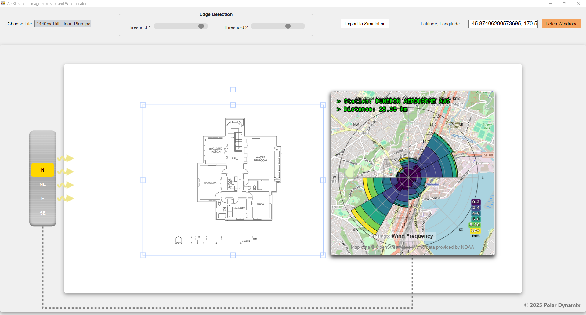
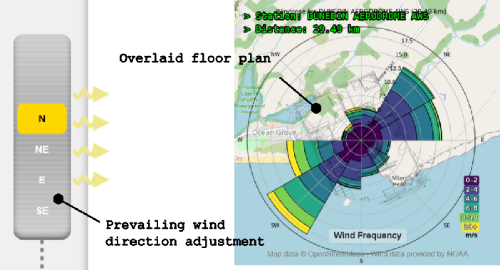
Image Setup and Wind Alignment

Users can load any image of interest — from a simple floorplan to an airfoil — into the simulation domain.

If needed, the system provides edge detection tools to help extract clear outlines from the image — especially useful when loading floorplans or sketches from the Internet.

Two sliders at the top of the interface control the edge detection threshold, allowing you to fine-tune what is considered an edge based on contrast. This ensures cleaner geometry recognition before simulation.

To simulate realistic wind exposure:

• Users can enter a latitude and longitude to retrieve wind data from the NOAA wind database.
• Use the prevailing wind direction wheel to set the wind origin.
  • For example, selecting SE means wind is blowing from the southeast, entering from the left side of the simulation domain.
• The floorplan is automatically overlaid on a wind rose, so as you rotate the wind wheel, you can see how your structure is oriented relative to real-world wind directions.

The tool offers two independent workflows:

• A. Prepare & Export Geometry — Trace and extract shapes from an image to use as CFD obstacles.
• B. Add Wind Data — Automatically retrieve and overlay wind patterns based on geographic coordinates.

a. Preparing and Exporting an Image

Open the Image Processor

• From the main AirSketcher interface, launch the “Image Processor & Wind Locator” module.

• A new window with a canvas-based UI will appear.

Load Your Image

• Click the file upload button (Choose File) to load an image (e.g. floorplan, sketch, aerial view).
• Supported formats: .jpg, .png, .bmp, etc.
• The image is automatically resized and centered.

Refine Image Outlines

Use the two sliders to control how clearly shapes and boundaries are extracted from your image.

• Lower slider values highlight faint lines and subtle features — ideal for hand-drawn sketches or soft scans.
• Higher values ignore minor details and emphasize bold, well-defined edges — best for high-contrast images.

The image preview updates in real time over a clean white background, giving you immediate feedback.

Export for Simulation

• When satisfied with the edge outlines:
  • Click “Export to Simulation”
  • This creates a saved_drawing.pkl file in your local project folder.
  • This file contains the extracted geometry for use in your CFD domain.

b. Adding Real Wind Data

Enter Coordinates

• Type latitude and longitude into the Latitude, Longitude box (e.g., 40.7128, -74.0060 for NYC).
• Press “Fetch Windrose”

What Happens Behind the Scenes

• The app finds the nearest NOAA weather stations using a built-in database.
• It downloads historical wind data.
• It automatically generates a windrose — a circular plot showing the most frequent wind directions and speeds.

Visual Map Overlay

• A high-resolution OpenStreetMap image centered on your location is downloaded.
• The windrose is automatically overlaid on the map, with frequency values shown.
• Your floorplan image is also overlaid on top of the windrose, for visual orientation.

Align with Wind

• Use the scrollable wind direction wheel on the left.
• Select a direction (e.g., “SW”) to rotate the canvas accordingly.
• The software auto-rotates and overlays your drawing.

Reading a Wind Rose

A wind rose is a visual summary of how wind speed and direction are distributed at a specific location.

Below is an example from DUNEDIN AERODROME AWS, approximately 41.95 km from the reference point.

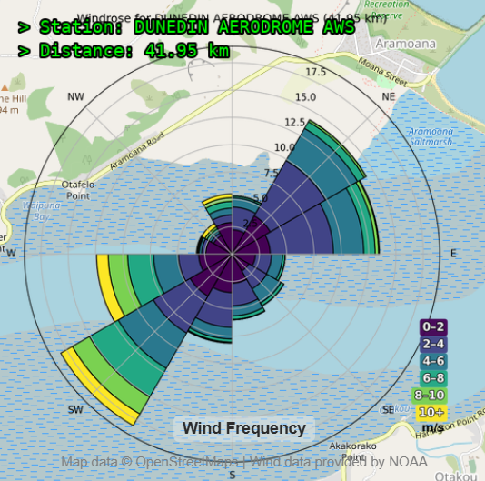
How to Read the Wind Rose:

• Direction (compass orientation): Each wedge shows where the wind comes from. For example, large bars pointing NE and SW mean wind frequently blows from NE and SW.
• Bar length: Longer bars = higher frequency from that direction.
• Color shading: Indicates wind speed ranges (legend at right):
  • 🟣 0–2 m/s
  • 🔵 2–4 m/s
  • 🟢 4–6 m/s
  • 🟡 6–8 m/s
  • 🟩 8–10 m/s
  • 🟨 10+ m/s
• Concentric rings: Represent frequency percentages (e.g., 2.5%, 5%, 10%, 15%, 17.5%)

Setting Wind Inputs in a Simulation

Wind Direction

• Use the dominant direction(s) — in this case:
  • Strongest wind comes from NE and SW
  • These are good candidates for inflow boundary direction

💡 Simulation Logic:
In the simulation environment, the wind always enters from the left side of the domain. This is because the software sets the inlet boundary on the left, with flow moving horizontally rightward.

What You Need to Do:
If wind in reality comes from NE (45°):

• Rotate your obstacle or layout so that wind enters from the left.
• Or use the wind direction wheel to rotate the layout accordingly.

Example:

If real wind is from SW (225°):

• Rotate the model layout so SW aligns with the left side
  
• Or set inlet direction to SW in the control panel

📌 Always align wind direction relative to the left-side inlet, since that’s where airflow begins.

Wind Speed

• Use the most frequent wind speed range
  • For this case: 4–6 m/s (green)
  • Suggested input speed: 5 m/s

Example Setup:

Wind direction: 45° (from NE) or 225° (from SW)
Wind speed (at a reference height 10m): 6 m/s

ℹ️ If using ABL (Atmospheric Boundary Layer), the 5 m/s typically applies at the domain top (e.g., 10 m or 100 m height).

Summary

When You’re Ready

• Return to the main simulation screen
• Use the Import image icon (right panel) to import your .pkl obstacle layout
• Click Run to begin simulation

Running a Simulation

Once your geometry, wind zones, and simulation parameters are set, running a simulation in AirSketcher is straightforward — though behind the scenes, the solver performs several intelligent steps to ensure stability, accuracy, and physical realism.

How to Start

1. Click the ▶ Run Simulation button.
   
2. The solver begins processing your setup: geometry, wind, zones, and any porous or blower definitions.
   
3. A live residual plot opens to monitor convergence.

What Happens During the Simulation

For each iteration, the solver performs:

• Time step (dt) calculation using the CFL condition:
  Lower CFL values are used when Refine Flow is enabled, improving accuracy.
• Porous and blower zones are applied to the velocity field.
• Velocity (u, v) and pressure (p) fields are updated, respecting all boundary conditions.
• Mass flow is balanced between inlets and outlets to avoid volume gain/loss.
• Residuals are computed to measure change between steps:

Residual_u = |u - u_prev|
 Residual_v = |v - v_prev|
 Residual_p = |p - p_prev|

These residuals are shown live in the solver graph.

Live Monitoring

Every 200 iterations (default, configurable):

• A Live Progress View updates:
  • Shows streamlines and velocity heatmaps.
  • Highlights high-interest zones.
  • Displays mass balance and a real-time Design Score based on airflow smoothness and coverage.

When the Simulation Stops

The solver now uses explicit, code-level criteria for stopping or notifying you:

• Convergence → Auto-Stop
  • Triggered only after the solver has run a minimum number of iterations (internal guard).
  • Mass flow imbalance (|ṁ_in − ṁ_out| / ṁ_in) < 1.00%.
  • All three step-change residuals (Ux, Uy, Pressure) fall below 0.005%
    (these are percent changes between successive iterations, not absolute field values).
  • When met, the solver stops automatically and shows a “Simulation Stopped” info message.
• Stagnation / Plateau → Non-blocking Notice (keeps running)
  • Over the last 100 iterations, the maximum change in each residual is < 1e-5, and mass flow imbalance < 1.00%.
  • You’ll see a non-blocking toast:
    “Residuals have plateaued—improvements are marginal and slow. Continuing run (iteration N).”
  • The simulation continues (no dialog to dismiss, no stop).
• Maximum Iterations Reached (20,000) → Prompt
  • At 20,000 iterations, you’ll be asked whether to continue.
  • If you choose Continue, the run proceeds and you won’t be prompted again in this run.
  • If you choose Stop, the solver ends.
• Divergence / Instability → Auto-Stop
  • If any residual spikes to an extreme value (e.g., > 10,000%) or mass flow imbalance > 200%, the solver stops automatically and shows a warning.

Other Insights

• CPU and RAM usage are displayed in the solver window.
• Total runtime is shown after simulation ends.
• Warnings are displayed if instability is detected, and the solver will auto-stop.

After Completion

• Simulation controls become re-enabled.
• You can review:
  • Final residual curves
  • Streamline, pressure, particle tracking visualizations
  • An innovative Qi Flow Index (QFI)
• You can modify any settings and rerun.

Notes

• The solver runs in steady-state mode (not time-dependent).
• Always rerun the simulation after changes to:
  • Geometry or boundaries
  • Inlet wind speed or direction
  • Zone types (porous or blower)
  • Mesh height or layout alignment

Solver behavior depends on: - Domain height (ly) - Inlet speed - CFL condition (automatically adjusted if Refine Flow is on)

💡 Pro Tip

Not sure if the simulation is stable?

Look at the residual plot:

• ✅ A steady downward trend with values close to zero means you’re converging.
• A flat or rising line suggests a problem — try:
  • Lowering the inlet speed
  • Enabling Refine Flow
  • Disabling AMR

Visualizing Results

After the simulation is complete, you can view the results using the panel of visualization tools. Each button provides a specific type of analysis to help interpret flow behavior, pressure distribution, or derived performance.

Velocity Contour

The Velocity Contour tool renders a filled color map of the fluid velocity magnitude across your simulation domain. It helps you spot high-speed regions, wake formations, and flow symmetry — all at a glance.

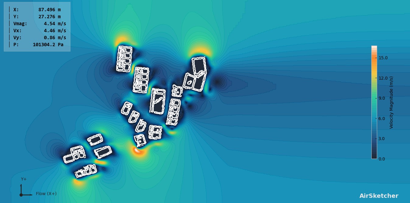
Features

• Colormap Customization
  Input your own min/max values to stretch or compress the contour color scale. This is especially useful when:

  • Focusing on low-velocity boundary layers
  • Comparing different cases side-by-side

• Interactive Hover Tooltips
  Hover anywhere on the plot to view:

  Vmag:  Velocity Magnitude (m/s)
   Vx:    Horizontal Component (m/s)
   Vy:    Vertical Component (m/s)
   P:     Static Pressure (Pa)

• Line Probe Tool
  Draw custom line probes to sample flow data across any two points. You’ll get:

  • Velocity & pressure plots
  • Vx/Vy component plots
  • Mass flow per segment
  • Exportable data tables

Usage Tips

• Use “Apply” to rescale the color range.
• Use “Streamlines”, “Particle Tracking”, or “Qi Flow” to explore complementary visualizations.
• Use “Report” to get an instant summary of your current simulation results.

📌 Notes

• Velocity in enclosed regions is automatically masked to avoid misleading visuals.
• Results are interpolated back onto the original grid, ensuring visual consistency.
• Watermark adapts brightness automatically for visibility across any background.

Streamlines

Streamline Analysis opens a clean, professional results window that shows high-quality streamlines colored by velocity magnitude, obstacle rendering, and an interactive Line Probe tool for detailed flow profiling.

When to Use Streamlines

• Understand overall flow patterns and recirculation zones
  
• Visualize how wind moves around buildings, terrain, or objects
  
• Extract precise velocity profiles along any line (great for validation or reporting)
  
• Compare flow behavior with/without AMR or different inlet conditions

How to Open

Click the Streamlines button in the Results panel (or use the toolbar icon).
A new window appears with a large, publication-ready visualization.

Main Visual Features

• Streamlines automatically colored by local velocity (m/s) using a beautiful aero/journal colormap
  
• Optional velocity vectors (arrows)
  
• Dark or Light theme (toggle anytime)
  
• Background mist effect for depth (in dark mode)
  
• Full Matplotlib toolbar (zoom, pan, save as PNG/PDF, etc.)

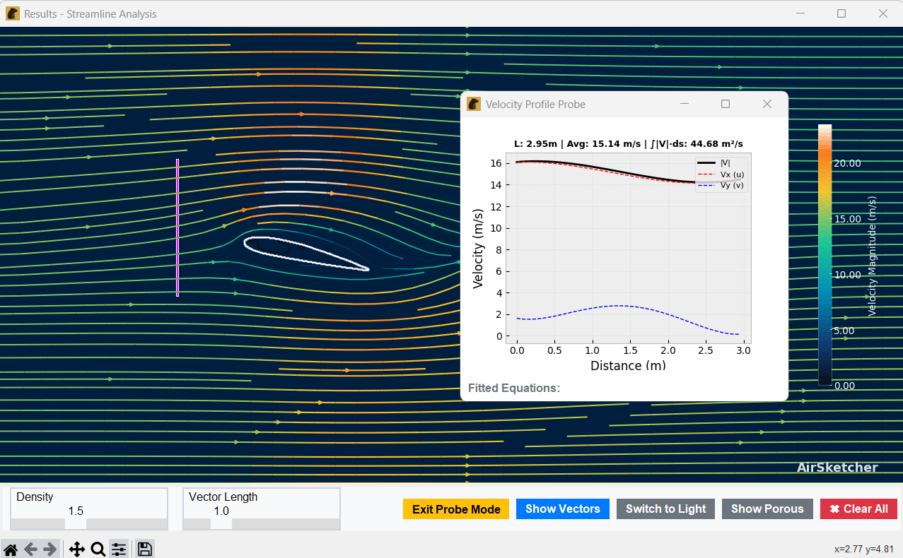#### Controls (bottom bar) - Density slider — controls how many streamlines are drawn (0.5 = sparse, 3.0 = very dense)
- Vector Length slider — scales arrow size when vectors are enabled
- Show/Hide Vectors — toggle velocity arrows on/off
- Switch Theme — Dark ↔︎ Light (journal quality)
- ⌖ Line Probe — activates the powerful profiling tool
- ✖ Clear All — removes probe lines and tooltips

Line Probe Tool (real time)

1. Click ⌖ Line Probe (button turns yellow).
   
2. Click and drag anywhere on the streamline map to draw a measurement line.
   
3. Release the mouse — a graph instantly appears showing:
   • |V| (velocity magnitude) — thick black line
     
   • u (horizontal) — red dashed
     
   • v (vertical) — blue dashed

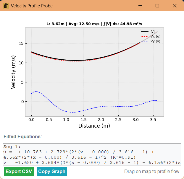Graph information displayed: - Total line length (m)
- Average velocity along the line
- Flux integral ∫|V|·ds (m²/s)

Fitted Equations (shown below the graph): - Automatic polynomial curve fitting with R² values
- Equations can be copied with right-click → Copy

Extra actions in probe window: - Export CSV — saves distance, u, v, |V| data
- Copy Graph — copies the plot image to clipboard (ready for reports)

Right-click anywhere on the main streamline map to clear all tooltips instantly.

Tip: Use the Line Probe on critical sections (e.g., above a roof, through a gap between buildings, or along a pedestrian path) to get exact numbers for your analysis or validation.

This tool turns raw simulation data into clear, presentation-ready flow insights in seconds.

Pressure Contours

The Static Pressure visualization shows how pressure is distributed throughout the simulation domain. It helps identify high-pressure stagnation zones, low-pressure suction regions, wake effects, and pressure loading around obstacles.

At a glance
Use Pressure Contours when you want to understand where air is pushing against a surface, where suction is forming, and how pressure differences contribute to aerodynamic force.

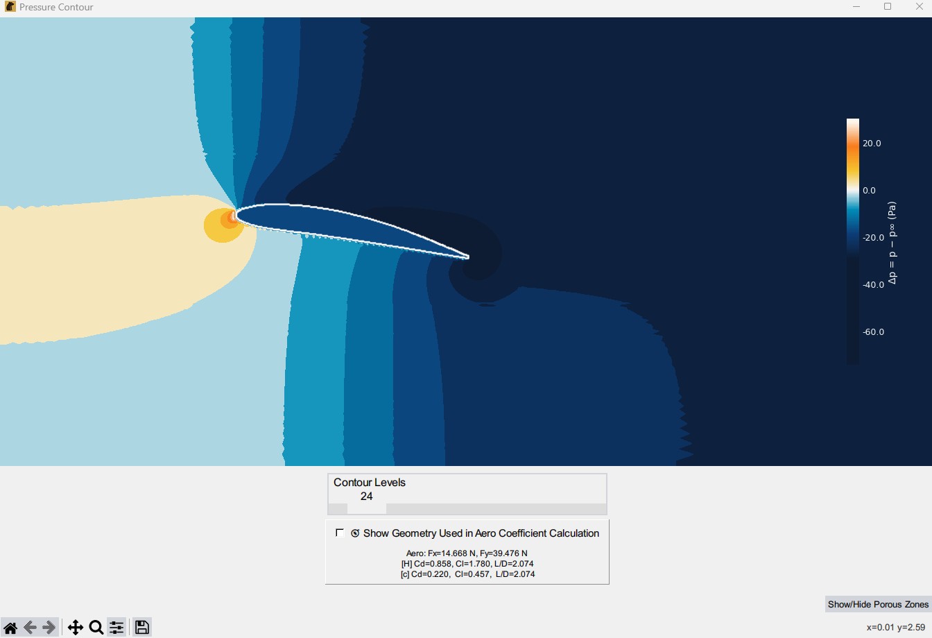
Key Features

• Pressure Contours
  High-resolution colored shading of pressure difference, shown as Δp = p − p∞, with optional black isolines.

• Value Tooltips
  Left-click anywhere in the fluid domain to display local Δp.
  Right-click clears all tooltips.

• Contour Detail Control
  Slider range: 5–250 levels.
  Use fewer levels for a clean overview and more levels for detailed pressure-gradient inspection.

• Geometry Overlay
  Toggle to show the detected outer obstacle boundary in green and the chord/reference line in red.

• Porous / Blower Zones
  Porous and blower regions are shown by default. Toggle them on or off to highlight forcing regions.

• Interactive Line Probe
  Draw any line across the pressure field to compute an integrated pressure-force estimate along that path.

How to Open & Use

Click the Pressure Contours button in the Results panel.

A large, clean window opens with the full Matplotlib toolbar for zooming, panning, and exporting.

Bottom controls:

• Contour Levels slider
• Show Geometry checkbox
• Show Isolines checkbox
• ⌖ Line Probe button
• Live Aero Data panel on the right side

Line Probe Tool

1. Click ⌖ Line Probe. The button turns yellow.
2. Click and drag a line across the pressure field.
3. Release the mouse button.
4. A new window appears with:
   • pressure profile graph;
   • smoothed curve and filled area;
   • total line length;
   • integrated force F [N/m];
   • direction angle;
   • fitted polynomial equations;
   • Export CSV and Copy Graph buttons.

This is useful for checking pressure distribution along a roofline, through a narrow gap, across a wake, or over a selected structural face.

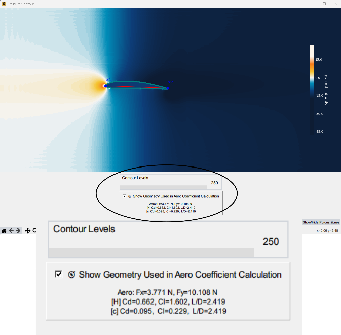
Aerodynamic Analysis

The software automatically detects the largest closed obstacle and estimates pressure-only aerodynamic force. This means the calculation uses pressure loading around the obstacle boundary, but does not include viscous shear stress.

Relative pressure field

p_rel(x, y) = p(x, y) − p∞ − bₓ(x − x₀) − bᵧ(y − y₀)

where: p_rel = corrected relative pressure p(x, y) = local static pressure p∞ = far-field or reference pressure bₓ and bᵧ = background pressure-gradient correction terms x₀ and y₀ = reference location

The background correction removes broad numerical pressure drift so the force calculation focuses on the pressure caused by the obstacle itself.

Force on each boundary segment

dF = −p_rel × n̂ × ds

where: dF = small force contribution from one boundary segment n̂ = outward unit normal vector ds = boundary segment length

Total force per unit span

F = ∮ over obstacle boundary [−p_rel × n̂ × ds]

The result is reported per unit depth out of the 2-D plane, so force units are N/m.

Advanced Features in the Calculation

• Voting raycast for correct outward normals, including concave and bluff bodies
• Automatic chord-line detection
• Automatic angle-of-attack detection
• Blockage correction when wind-tunnel mode is active
• Time-averaging filter for more stable force estimates during vortex shedding
• Calibration multiplier for matching experimental or reference data

Important note
This is a pressure-only aerodynamic estimate. For many 2-D bluff-body cases, pressure force dominates the total force, but viscous shear is not included.

Aerodynamic Coefficients

The software converts force into dimensionless aerodynamic coefficients using dynamic pressure.

Dynamic pressure

q∞ = 0.5 × ρ × U∞²

where: q∞ = dynamic pressure ρ = air density U∞ = reference freestream velocity

Using Projected Height [H]

Use this convention for bluff bodies, buildings, cylinders, and objects where the projected frontal height is the most meaningful reference length.

Height-based coefficients

CD[H] = Fx / (q∞ × H)
CL[H] = Fy / (q∞ × H)
L/D[H] = CL[H] / CD[H]

where: H = projected height Fx = streamwise force per unit span Fy = vertical force per unit span CD[H] = drag coefficient based on projected height CL[H] = lift coefficient based on projected height

Using Chord or Streamwise Length [c]

Use this convention for airfoils, streamlined bodies, and wind-tunnel-style analysis where chord length is the standard reference.

Chord-based coefficients

CD[c] = Fx / (q∞ × c)
CL[c] = Fy / (q∞ × c)
L/D[c] = CL[c] / CD[c]

where: c = chord or streamwise reference length CD[c] = drag coefficient based on chord CL[c] = lift coefficient based on chord

Both coefficient sets appear live in the Aero Data panel.

The panel includes:

• Fx / Fy [N/m]
• Angle of attack, AoA
• Reynolds number, automatically selected based on body thickness
• Height-based coefficient set, [H]
• Chord-based coefficient set, [c]
• Optional manual calibration using Set [H] or Set [c]

How to Interpret the Pressure Plot

• High pressure in front of an object usually indicates stagnation, where flow slows down and pushes against the surface.
• Low pressure around corners or roof edges often indicates suction and acceleration.
• Large pressure differences across an object usually indicate higher aerodynamic loading.
• Oscillating pressure regions behind an object can indicate wake formation or vortex shedding.
• Strong pressure gradients through gaps may indicate jetting, channeling, or local acceleration.

Accuracy Tips

• Keep at least around 4 to 5 × body height clearance from domain boundaries when possible.
• Avoid placing the object too close to the inlet, outlet, top, or bottom boundary.
• Use Wind Tunnel Mode only when a confined tunnel-style setup is intended.
• Use an open boundary setup for outdoor building or terrain studies.
• Let the simulation stabilize before recording final aerodynamic values.
• For aerodynamic coefficients, wait until residuals, mass balance, and ΔCd are stable.
• Use manual calibration only when you have trusted experimental or reference data.

Particle Tracking & PM2.5 Pollution Analyzer

New launcher — Click the Particle Tracking button to open a clean mode selector:

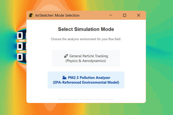
• General Particle Tracking (Physics & Aerodynamics) — classic tracer dots + optional smoke overlay
  
• PM2.5 Pollution Analyzer (EPA-referenced environmental model) — quantitative PM2.5 concentration mapping, sources, filters, and ESG/WHO reporting

Both modes use your current velocity field. Choose the one you need.

General Particle Tracking (original mode)

Visualises flow with animated tracer particles and an optional Smoke overlay (unitless normalised density map).

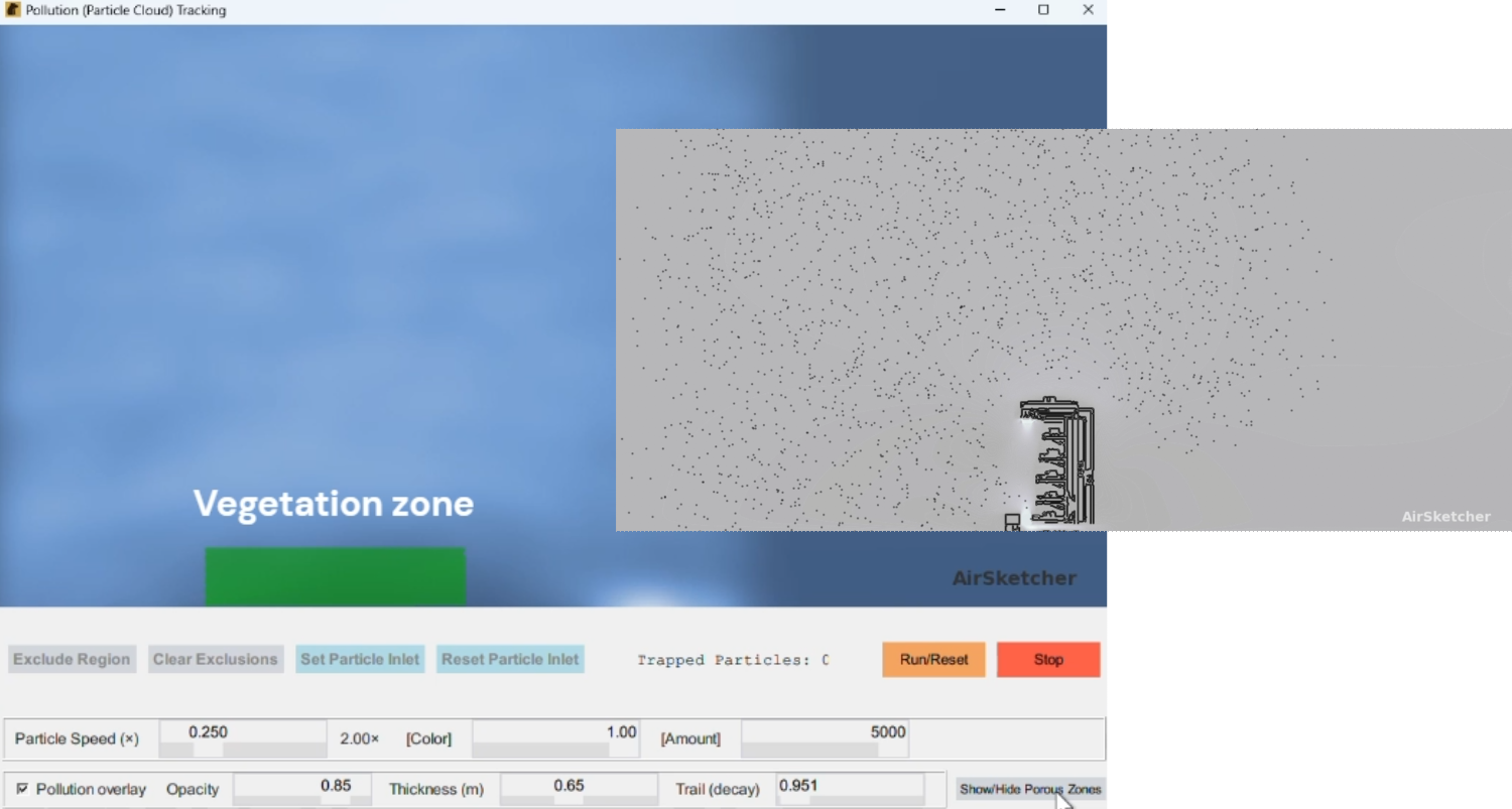
Features - Particles injected from the left inlet (or your custom polygon inlet) - Advected with velocity + tiny random walk for natural look - Red dots = stuck particles (speed < 0.001 × reference speed); live counter shown - Exclude Region polygons (counting only) — particles inside are ignored for trapping statistics but still move normally - Smoke overlay (when enabled) hides the dots for a clean plume view

Controls (bottom bar) - Particle Speed (×) – visual time scale - Color – dot brightness - Amount – number of particles - Smoke overlay toggles: Opacity, Thickness (m), Trail (decay), Theme (Blue Cloud / Smoke / Toxic Gas / Heatmap) - Buttons: Run/Reset, Stop, Exclude Region, Clear Exclusions, Set/Reset Particle Inlet, Show/Hide Porous Zones

Smoke Overlay mathematics (for advanced users) The overlay is built on the simulation grid:

1. Bilinear deposit of particle footprints → fresh deposit D
2. Compact Gaussian blur (controlled by Thickness)
3. Trail memory: C(k+1) = α·C(k) + D̃ (α from Trail slider)
4. Outlet sponge + solid masking
5. Normalised display with running 98th-percentile EMA + gamma ≈ 0.72

Tooltip always shows Pollution: XX% (normalised intensity, no physical units).

Reading values - Left-click in fluid → “Pollution: XX%” - Right-click → clear all tooltips

When to use
Perfect for visualising recirculation, stagnation zones, or qualitative ventilation studies.

PM2.5 Pollution Analyzer (pro mode)

Full quantitative environmental modelling with real concentrations in µg/m³, source emissions, filters, Zone of Interest statistics, WHO compliance panel, and one-click ESG reporting.

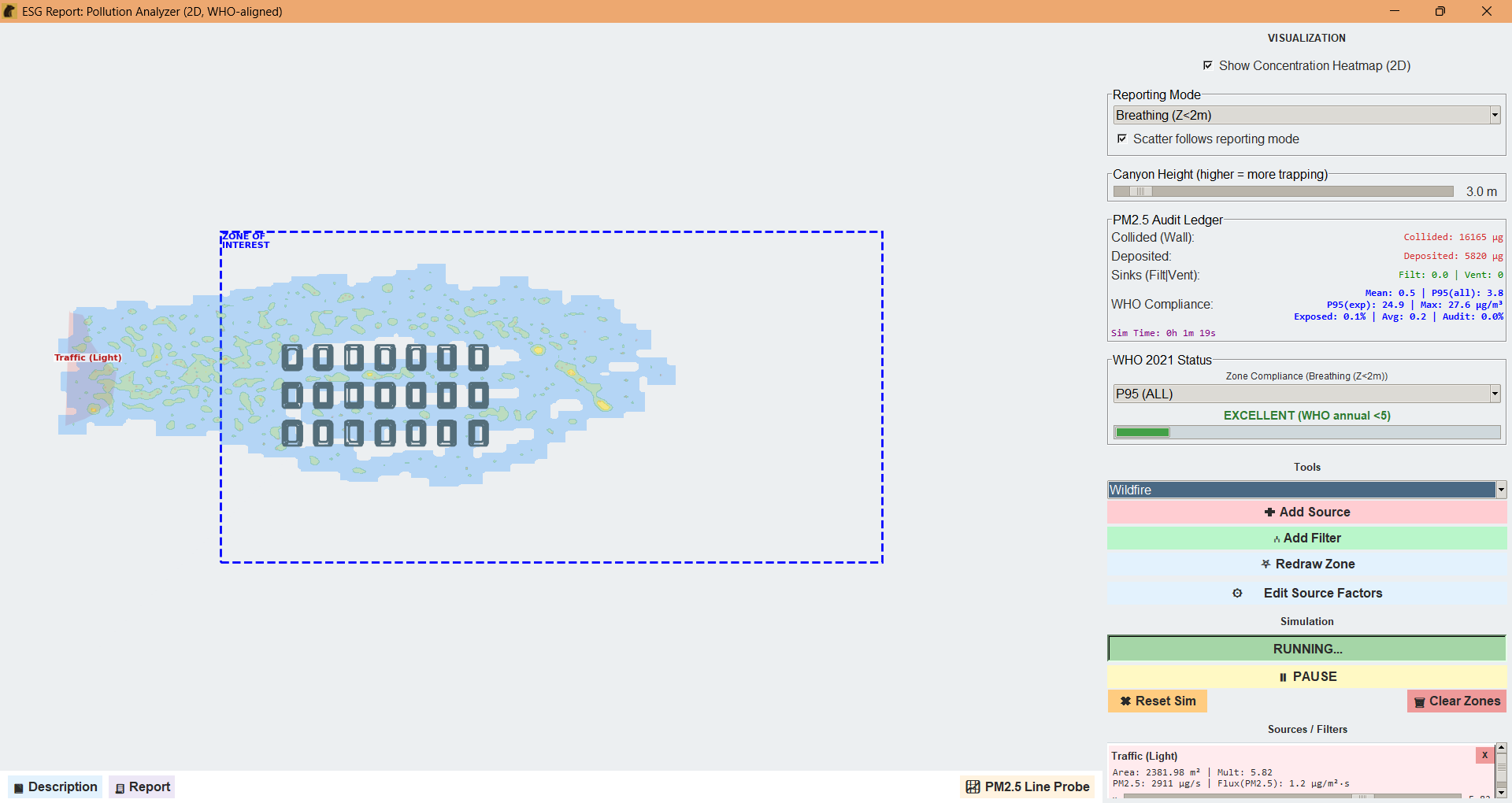
Key Features

• Heatmap — coloured concentration field (µg/m³) built from airborne PM2.5 mass only (deposited mass is excluded)
• Reporting Mode — choose Breathing (Z<2m) (near-ground exposure) or Column Proxy (taller mixing-height average). Physics always runs on full 3D particle state; reporting mode only changes what is counted for the map and statistics
• Scatter follows reporting mode checkbox — filters the visible particle dots to match the reporting mode (reduces clutter in Breathing view) while the heatmap always uses the selected mode
• Sources — draw polygons and assign real emission rates (µg/s), PM2.5 fraction, removal/decay, settling velocity, and height bias. Multiplier slider per source
• Filters — green polygons that remove particles (mass counted as “filtered”)
• Zone of Interest (blue dashed box) — defines the compliance region for all statistics
• Canyon Height — increases near-ground trapping in street-canyon scenarios
• PM2.5 Line Probe — draw any line on the map for a precise concentration profile (graph + CSV export)

Live Dashboard (right sidebar)

• Mean, P95 (all), P95 (exposed), Max, Exposed %, 24h-style average
• WHO 2021 status panel with colour-coded progress bar (Excellent / Good / Exceeds)
• Mass audit ledger: emitted vs (airborne + filtered + vented + collided + deposited + decayed)
• Sim time display

Buttons (under the plot)

• Description — opens a full printable explanation of every control and equation
• Report — generates a clean ESG PDF-ready report with embedded snapshot, audit ledger, and disclaimers
• PM2.5 Line Probe — activates the interactive concentration profiler

Accuracy & Scope - Qualitative-to-quantitative visualisation tool (not a certified regulatory model) - Concentrations are reconstructed via cloud-in-cell deposition + smoothing + division by reporting-layer volume - All mass bookkeeping is audited in real time for closure

Performance tips - Disable the heatmap temporarily while adding many sources/filters - Use moderate particle amounts (the simulator auto-culls excess for stability) - The line probe and dashboard update instantly — no extra waiting

When to use - ESG/sustainability reporting - “Before vs after” filter or source relocation studies - WHO compliance screening - Visualising PM2.5 hotspots and exposure zones

Why two separate modes?
General mode is fast and beautiful for flow insight. PM2.5 mode adds full emission → concentration physics, regulatory metrics, and professional reporting — all while sharing the same accurate velocity field.

Both tools are production-ready and export perfectly to HTML/PDF. Use the Description and Report buttons inside the PM2.5 Analyzer for complete technical documentation and formal outputs.

Line Probe

The Line Probe tool extracts precise values across any two points, or along a multi-point polyline, in the flow domain. It is useful for checking velocity variation, pressure change, mass-flow balance, and integrated velocity metrics along a user-defined path.

At a glance
The Line Probe samples flow variables along a drawn path and automatically reports distance-based plots, segment-wise mass flow, and integrated velocity metrics such as ∫ U ds, ∫ U² ds, and ∫ U³ ds.

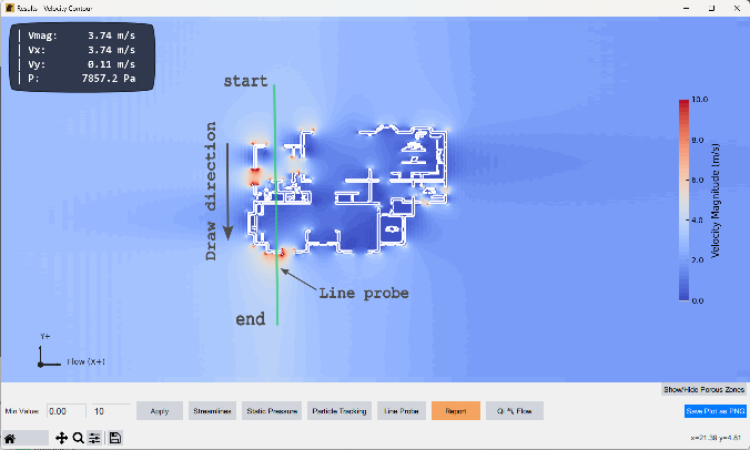
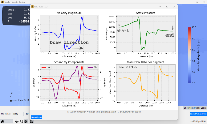
Steps

1. Start Probe
   Click Line Probe, then draw a polyline along the path you want to sample.

2. Reference Scaling (distance calibration)

   • If your domain axes are already 1:1 in meters, press OK in the dialog. No calibration is needed.
   • If your domain is scaled from pixels, CAD, or an image, draw a short reference line over a feature with a known real-world length, then enter that length in meters.
   • This sets the meters-per-unit scale so distances, mass flow rate, and integrated values are computed correctly.

Common integrated values
∫ U ds = integral of velocity
∫ U² ds = integral of velocity squared
∫ U³ ds = integral of velocity cubed

3. Auto Plots
   The tool automatically generates:
   • Velocity Magnitude vs Distance
   • Static Pressure vs Distance
   • Vx and Vy Components vs Distance
   • Mass Flow per Segment
   Distance is shown in meters using the scale from Step 2.

Mass-flow relation
ṁ = ρ × Vₙ × A

where: - ṁ is mass flow rate - ρ is fluid density - Vₙ is velocity normal to the line segment - A is the segment area, or effective segment width in the 2-D model

4. Interactive Table
   Shows sampled data:
   • X
   • Y
   • V
   • P
   • Vx
   • Vy
   • ṁ
5. Save
   Export the composite PNG plot.

Graph (Line Probe) Description

This section explains what each line-probe graph shows and how the summary numbers are computed.

You draw a polyline, and the tool resamples the field along its arc length from the start point to the end point.

Symbols used in this section

• s = distance along the polyline
• L = total polyline length
• Δsᵢ = local segment length
• uₓ = x-direction velocity component
• uᵧ = y-direction velocity component
• U = velocity magnitude

Velocity magnitude definition
U = sqrt(uₓ² + uᵧ²)

Raw vs Smoothed Curves

Each plot can show raw samples and a gently smoothed curve.

• Raw samples are the direct values taken from the solver field.
• Smoothed curves are display curves used to make trends easier to read.
• Integrals labeled raw are calculated from the unsmoothed samples.
• Integrals labeled smoothed are calculated from the displayed curve.
• The exported data table always contains the raw samples.

Important
Use the raw values for numerical checking and the smoothed curve for visual interpretation. Small differences between raw and smoothed integrals are normal.

Velocity Magnitude U [m/s]

• Curve: U(s) versus distance s.

Integrals shown in the lower-right badge

∫ U ds [m²/s]
∫ U² ds [m³/s²]
∫ U³ ds [m⁴/s³]

Optional mean velocity
U_mean = (1 / L) × ∫ U ds

• Notes:
  • ∫ U ds gives an accumulated velocity-length measure along the path.
  • ∫ U² ds is kinetic-energy-like and highlights faster regions.
  • ∫ U³ ds heavily weights velocity peaks and can be used as a proxy for transport potential, especially in sand or dust movement studies.

Example: Using a Near-Surface Line Probe and ∫ U³ ds for Sand Transport

Goal: Estimate along-line aeolian sand transport over 2-D topography using Bagnold-style cubic velocity scaling and the line-probe metric ∫ U³ ds.

1) Bagnold Scaling

Bagnold form used here
q = C × (ρ / g) × sqrt(d / D) × u∗³

Where:

• q = sand mass flux per unit width [kg/s/m]
• ρ = air density
• g = gravitational acceleration
• d = grain size
• D = reference grain size
• u∗ = friction or shear velocity
• C = empirical coefficient

Coefficient C

A practical range is: - C ≈ 1.5 for uniform, well-sorted sand - C ≈ 2.8 for widely graded sand

Practical tip: Start with C = 2.0, then calibrate against measured fluxes if field data are available.

2) Link u∗ to Measured Wind Speed U

Assume a log-law profile at a fixed near-surface reference height.

Definitions

• z_ref = reference height
• z₀ = roughness length
• κ = von Kármán constant, approximately 0.40

Log-law relation
U(z_ref) = (u∗ / κ) × ln(z_ref / z₀)

Solving for friction velocity
u∗ = κ × U(z_ref) / ln(z_ref / z₀)

3) Combine Bagnold Scaling with the Log Law

Combined form
q = K × U³

where

K = C × (ρ / g) × sqrt(d / D) × [κ / ln(z_ref / z₀)]³

If z_ref and z₀ are uniform along the probe, then K is constant.
If roughness changes strongly along the line, use a local value:

Kᵢ = local K for segment i

4) Draw a Polyline Line Probe Along the Near-Surface Path

Let the sampled vertices be (xᵢ, yᵢ) and the local arc-length spacing be Δsᵢ.

Tool metric

∫ U³(s) ds ≈ Σ(Uᵢ³ × Δsᵢ)

This means the line probe adds the cubic velocity contribution from each segment along the drawn path.

5) Convert the Metric to Transport

Total along-line transport

Q_line ≈ K × ∫ U³ ds

With SI inputs in K, the result Q_line is in kg/s.

6) Optional Threshold for Motion

If a threshold friction velocity applies, segments below the threshold should be set to zero.

Threshold definitions

• u∗t = threshold friction velocity
• U_t = equivalent threshold wind speed at the reference height

Threshold wind speed

U_t = (u∗t / κ) × ln(z_ref / z₀)

Thresholded transport estimate

Q_line ≈ K × Σ[max(Uᵢ³ − U_t³, 0) × Δsᵢ]

Assumptions / Tips

Assumptions and practical tips

• Use one consistent z_ref along the polyline when possible.
• Keep the probe above the roughness sublayer.
• If z₀ varies strongly, treat K locally as Kᵢ.
• Choose d and C for the expected sand type.
• The method is most appropriate for dry, non-cohesive sand.
• The ∫ U³ ds metric is a proxy for the Bagnold driver. Larger values indicate stronger transport potential along the drawn path.

Static Pressure p [Pa]

• Curve: p(s) versus distance s.

Pressure summary

∫ p ds [Pa·m]

Optional mean pressure
p_mean = (1 / L) × ∫ p ds

• Note: This is a line measure along the probe. It is not a surface force by itself.

Velocity Components uₓ and uᵧ [m/s]

• Curves: uₓ(s) and uᵧ(s) versus distance s.

Component note
The components can be positive or negative. The velocity magnitude U is always non-negative.

These component plots are useful for identifying flow reversal, recirculation, jet direction, and cross-flow behavior.

Mass Flow Across the Polyline [kg/s]

Let:

• ρ = fluid density
• n(s) = unit normal vector of the polyline, pointing to the measured side
• nₓ = x-component of the unit normal
• nᵧ = y-component of the unit normal
• Vₙ(s) = velocity normal to the polyline

Normal velocity

Vₙ(s) = uₓ(s) × nₓ(s) + uᵧ(s) × nᵧ(s)

Mass-flow density per unit length

ṁ′(s) = ρ × Vₙ(s)
Units: kg/s/m

Per-segment mass flow

ṁᵢ = ρ × Vₙᵢ × Δsᵢ
Units: kg/s

What Is Plotted

The mass-flow graph can show either:

• ṁ′(s) versus distance s, or
• per-segment totals ṁᵢ

Recommended display
ṁ′(s) versus s

This makes it easier to see where flow crosses the line most strongly.

Totals Shown in the Badge

Raw sum, discrete

Σ = Σ(ρ × Vₙᵢ × Δsᵢ)
Units: kg/s

This is the conservation check and matches the data table.

Continuous integral

Integral mass flow = ∫ ṁ′(s) ds
Units: kg/s

This is computed over the displayed curve, either raw or smoothed depending on the label. Small differences from the discrete sum are normal when smoothing or resampling is applied.

Units Sanity Check

Quick unit check

ρ [kg/m³] × Vₙ [m/s] × Δs [m] = kg/s
ṁ′ = ρ × Vₙ → kg/s/m
∫ ṁ′ ds = kg/s

U [m/s] × length [m] = m²/s
U² [m²/s²] × length [m] = m³/s²
U³ [m³/s³] × length [m] = m⁴/s³

Report & Analysis

The Report tool builds a polished, ESG-ready PDF and a Word-friendly bundle from your current simulation. It combines the selected Region of Interest (ROI), named Points of Interest (POIs), cross-design .pkl comparisons, and an integrated energy calculator to generate flow statistics, efficiency charts, carbon metrics, and AI-assisted engineering narratives.

The purpose of this report is to help users move from CFD visualization to practical engineering decisions: identifying whether a design improves airflow delivery, reduces resistance, supports fan speed reduction, improves outdoor-air effectiveness, or reveals hidden energy penalties.

Workflow

1. Run a simulation: Ensure velocity and pressure fields are fully established.
2. Open AI Analysis: Click Report / AI Analysis. A new window opens showing the current velocity map.
3. Draw the ROI: Drag a rectangle over the core area you want analyzed. Click Confirm ROI.
4. Pick POIs (points to sample): Click on the plot to drop one or more POIs. They will be numbered automatically. Click Confirm Points of Interest.
5. Name the POIs: A Name Zones window appears. Rename them using clear engineering labels such as Inlet Corner, Work Zone, Return Exhaust, or Filter Face. Click Submit.
6. Enter ESG & Comparison Data: An Energy & Carbon Inputs window appears.
   • Enter baseline operating data such as Fan Power (kW), Operating Hours, Baseline CFM, Electricity Tariff, and Grid Emission Factor.
   • Use After CFM only when a measured or known post-improvement airflow value is available.
   • Leave After CFM blank when comparing design-stage simulations and allowing AirSketcher to estimate performance from the r trends.
   • Cross-Design Comparison: Load up to two saved .pkl state files to directly compare alternative designs against the current baseline.
   • Click Use Values, or click Skip to leave ESG values as N/A.
7. Save the PDF: Choose a filename. AirSketcher generates the PDF in a high-contrast Soft Grid theme, creates a bundle folder, and automatically opens the folder.

What the Report Includes

• 1. Executive Summary & Introduction: Quick directional statistics including ROI mean/variance, key percentiles (P10/P50/P90), best/worst POI percentages, main flow direction, and reversed-flow area fractions.
• 2. Methodology & Theory: A clear layout of the solver configuration, featuring identically sized Governing Equations: Continuity, Momentum, PPE, and Spalart–Allmaras. The section also includes an ASCII boundary-condition sketch and automatically adds Porous/Blower equations, ABL profiles, and AMR mesh illustrations when active.
• 3. Results:
  • 3.1 Velocity & Streamlines: Side-by-side maps using the same color scale, with the ROI box and POI markers cleanly overlaid.
  • 3.2 ROI Statistics: Histogram and Cumulative Distribution Function (CDF) of velocity within the selected ROI.
  • 3.3 & 3.4 POI Data: Data tables and bar charts comparing velocity and static pressure at each named POI.
• 4. Energy & Carbon Savings (ESG-Ready):
  • 4.1 Calculations: Translates flow improvements into hard numbers using Fan Affinity Laws, Outdoor-Air (OA) reduction estimates, and Thermostat Setpoint shifts.
  • 4.2 Savings: Breaks down Fan, OA, and Setpoint savings into kWh/yr, Cost/yr, and tCO2e/yr.
  • 4.3 Cross-Design Comparison: If .pkl files are loaded, this section compares them using a CFM proxy ratio, r. It generates a Standard Table for downstream/supply POIs and an Upstream Table using a pressure-drop proxy for return, exhaust, filter, and suction-side evaluation.
  • 4.4 Energy ROI Interpretation Guide: Adds a deeper explanation of when airflow changes represent real energy savings, when they indicate resistance penalties, and which calculation recipe should be used.
• 5. Conclusions: Explains how to interpret the performance ratio r based on whether POIs are upstream or downstream of the fan. It also provides actionable engineering next steps for design optimization, fan control, resistance reduction, and ESG reporting.

Section 4 Extension: Energy ROI Interpretation Guide

The Energy & Carbon section should be interpreted using one central rule:

AirSketcher does not save energy automatically. It identifies the aerodynamic opportunity. Energy is saved only when the design is improved and the controls are adjusted to use that improvement.

This distinction is important because low airflow can mean two very different things.

4.4.1 Downstream Performance Ratio

For supply, cooling, and occupied-zone POIs, AirSketcher uses the downstream performance ratio:

r = V(new) / V(baseline)

Use this interpretation:

When r > 1 downstream, the report estimates fan savings using the Fan Cube Law:

P ∝ N³

This means a small reduction in fan speed can create a much larger reduction in fan power. If a design delivers the same target airflow at a lower fan speed, annual energy and carbon savings can become significant.

4.4.2 Upstream / Exhaust Performance Ratio

For upstream, return, exhaust, hood, filter, or suction-side POIs, velocity alone is not enough. A blocked filter may show lower airflow, but that does not mean energy is being saved. It may mean the fan is working harder against resistance.

For this reason, AirSketcher uses a fan power proxy:

Power Proxy ≈ rQ × rDP

Where:

• rQ is the flow ratio.
• rDP is the pressure-drop ratio.

Use this interpretation:

This is especially useful for diagnosing dirty filters, clogged return paths, restrictive exhaust hoods, and poor inlet conditions.

4.4.3 The Four Energy-Saving Recipes

AirSketcher organizes energy savings into four practical recipes. Select the one that matches the engineering goal of the project.

4.4.4 Required Inputs for Valid Financial Outputs

The ESG section requires complete input data. If required values are missing, the report will still generate, but cost and carbon fields may show --.

Universal inputs:

Airflow input options:

4.4.5 Dirty Filter / Resistance Example

A common mistake is assuming that constant airflow means constant energy. For example, a fan system with a dirty filter may maintain the same target velocity because the VFD increases fan effort.

In the simulation, the airflow may look acceptable, but the pressure drop can rise sharply. In this case:

• rQ ≈ 1.0 means the airflow is being maintained.
• rDP > 1.0 means pressure drop has increased.
• A higher power proxy means the fan is spending more energy to overcome resistance.

This is not a saving. It is a hidden energy penalty.

For filter banks, return inlets, and exhaust systems, the Upstream Table is therefore more important than the Standard Table because it captures the combined effect of flow and pressure drop.

4.4.6 Outdoor-Air Reduction Logic

Outdoor air is expensive to condition because it must be cooled, heated, or dehumidified before entering the occupied space.

If the ROI statistics show better mixing, lower variance, and improved low-percentile velocity behavior, the report may estimate a conservative outdoor-air reduction. This is especially useful when the Outdoor-air after field is left blank but a comparison .pkl file is provided.

The automatic estimate is intentionally conservative and capped at 20% for safety. This prevents the report from overstating savings where ventilation compliance, process requirements, or local codes still control the minimum outside-air requirement.

4.4.7 Thermostat Setpoint Shift Logic

If the simulation shows fewer stagnant zones, fewer hot spots, and a more uniform air distribution pattern, the building may not need to be over-cooled to fix one poor-performing area.

In this case, the report can estimate savings from a thermostat setpoint shift. For example, raising the cooling setpoint by 1°C can reduce cooling demand while maintaining more consistent comfort or process conditions.

This calculation is most useful for:

• climate-controlled warehouses;
• manufacturing floors;
• production rooms;
• large open-plan facilities;
• spaces where one hot zone causes the entire system to over-cool.

4.4.8 How to Use Section 4 in Client Discussions

Use Section 4 to separate visualization from action.

A velocity plot shows where air moves.

The ESG section explains what the movement means financially.

The key client message is:

The simulation identifies where the airflow system is inefficient. The savings are realized when the improved design is combined with the correct operational action, such as reducing fan speed, lowering outdoor-air load, cleaning resistance points, or adjusting the thermostat setpoint.

This makes the report useful for engineering review, financial justification, ESG documentation, and before/after design comparison.

Outputs

• PDF Report: The final document, styled in a professional BlueGray palette with zebra-striped tables.
• Bundle Folder: Auto-created next to the PDF. It contains all high-resolution PNG images used in the report, plus a report_insert.docx or .md file so the findings can be copied into company documents.
• AI Pack (.json): A single compressed JSON file containing arrays, grid data, boundary conditions, and embedded images. This can be provided to an AI assistant to generate a custom engineering summary based on the raw CFD data.

Notes & Tips

• Mandatory POIs: You must pick at least one POI to proceed. Grouping POIs with the exact same name will automatically average them together as a Zone in the final tables.
• Use Clear POI Names: Names such as Supply Target, Return Intake, Filter Face, Worker Zone, and Exhaust Hood make the final report easier to interpret.
• Downstream vs Upstream Matters: Use downstream interpretation for supply and occupied-zone performance. Use upstream interpretation for return, exhaust, suction, filter, and hood evaluation.
• Auto-Estimated OA: If the Outdoor-air after field is left blank and a comparison .pkl file is provided, the report can estimate a conservative OA reduction based on ROI variance and P10 dead-zone improvement, capped at 20%.
• Interpreting Proxy Ratio r: An r > 1 downstream usually means better delivery to the target zone. An r > 1 upstream can mean higher pressure drop or resistance, which may be bad. The Conclusions section explains this distinction for client-facing interpretation.
• Energy Requires Action: Energy savings are only realized when the aerodynamic improvement is paired with an operational change, such as fan speed reduction, resistance removal, outdoor-air adjustment, or thermostat setpoint change. ### Qi-Flow

Qi-Flow (QFI) blends CFD with Feng Shui to assess air harmony, clarity, and comfort.

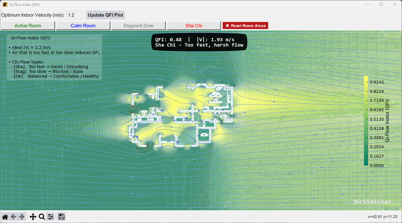
How QFI Works

• $|V| = \sqrt{u^2 + v^2}$
  
• V_opt = 1.2 m/s (target)
  
• σ = 0.6 m/s (tolerance)

Formulas:

• Smoothness
  $$ S = \frac{1}{1 + \nabla |V|} $$

• Comfort
  $$ V_s = \exp\left(-\frac{(|V| - V_{\text{opt}})^2}{2\sigma^2}\right) $$

• Qi-Flow Index
  QFI = S × V_s

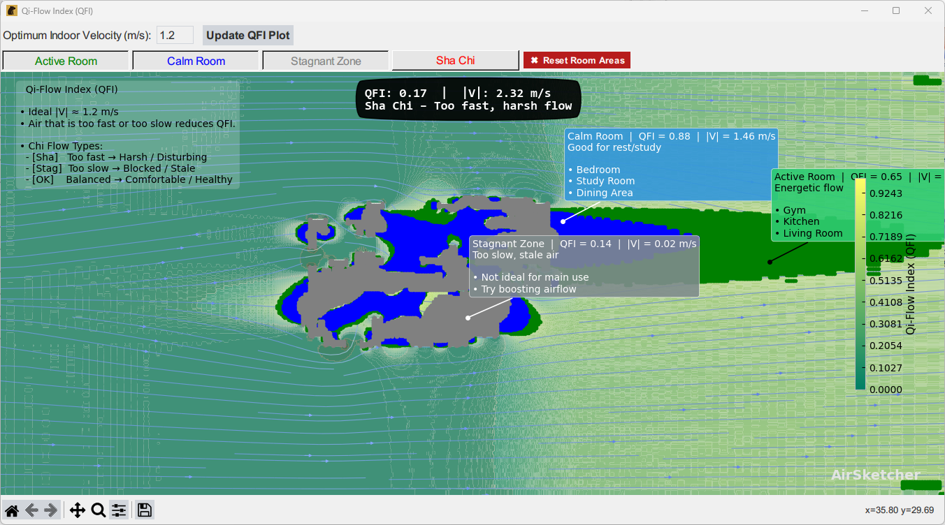
Room Classification

Tips for Qi-Aligned Flow

• Break long corridors with buffer zones (read more)
• Allow air to circulate in loops between zones (read more)
• Favor gentle curves over sharp corners (read more)
  
• Enable Refine Flow for natural transitions
  
• Consider adding trees or vegetation zones in outdoor or semi-enclosed areas to introduce soft flow resistance and improve harmony (read more)

👥 Credits

Core Development

• Tech Architect: Dr. Wichai Pattanapol
  
• Head of Client Relationships: Adam Gill

🔖 Licensing & Acknowledgements

AirSketcher may incorporate open-source components under compatible licenses.
All third-party libraries retain their original licensing terms.

📨 Contact

For questions, feedback, or collaboration inquiries:

📧 support@polar-dynamix.com
🌐 www.polar-dynamix.com